library(tidyverse)
# let's remove any labels and scales
theme_set(theme_void() + theme(legend.position = "none"))Getting started
This quick start guide is largely inspired from the excellent workshop by Danielle Navarro.
(Optional) recording the making of the plot
library(camcorder) # optional! For getting the gif at the end.
gg_record(
  dir = file.path(tempdir(), "recording"), # where to save the recording
  device = "jpeg", # device to use to save images
  width = 4,      # width of saved image
  height = 4,     # height of saved image
  units = "in",   # units for width and height
  dpi = 300       # dpi to use when saving image
)
Start with any data you like, but we are going to plot the data in the mtcars dataset. We can start with some simple scatter plot.
ggplot(mtcars, aes(wt, disp, color = factor(am))) +
  geom_point(size = 5) +
  scale_color_manual(values = c("skyblue", "orange"))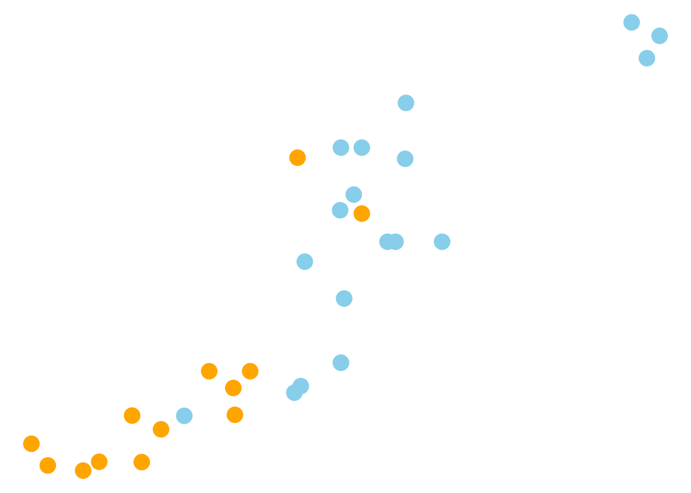
Now let’s have some fun!
g1 <- ggplot(mtcars, aes(wt, disp))  +
  geom_segment(aes(xend = 0, yend = 0, linewidth = hp)) +
  geom_point(size = 5, color = "black", aes(wt - 0.02, disp - 1)) +
  geom_point(aes(color = factor(am)), size = 5) +
  scale_color_manual(values = c("skyblue", "orange")) +
  scale_linewidth_continuous(range = c(0.05, 1))

g1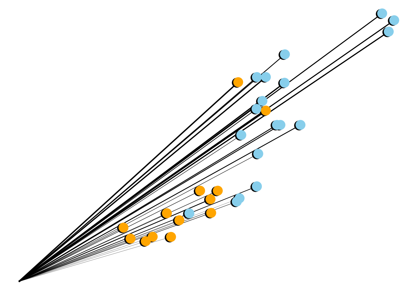
g1 + coord_polar()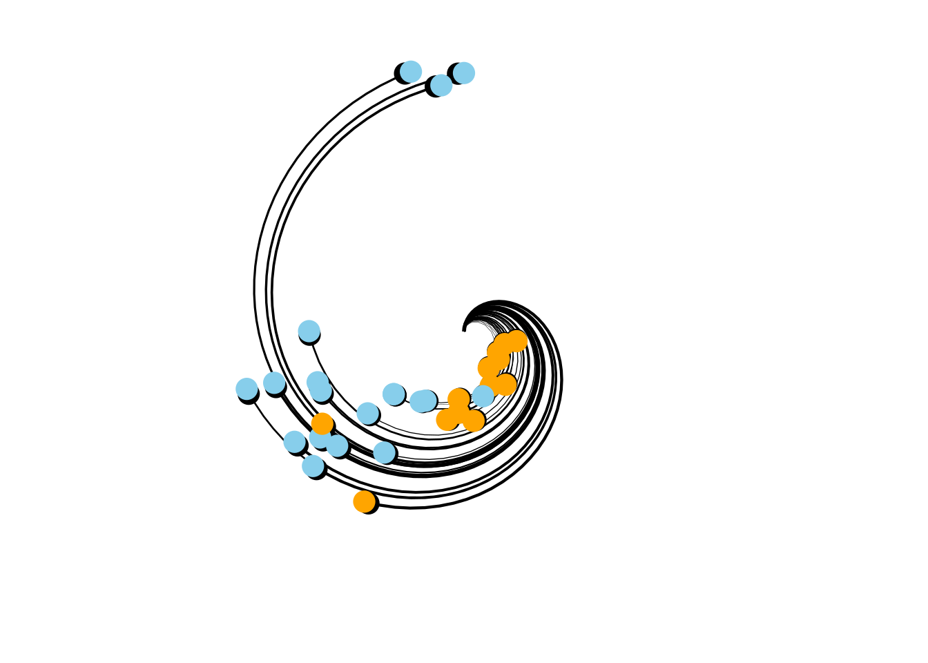
g1 +
  coord_polar("y") +
  annotate("point", size = 20, x = 0, y = 0) +
annotate("point", size = 3, x = 0.5, y = 1, color = "white") 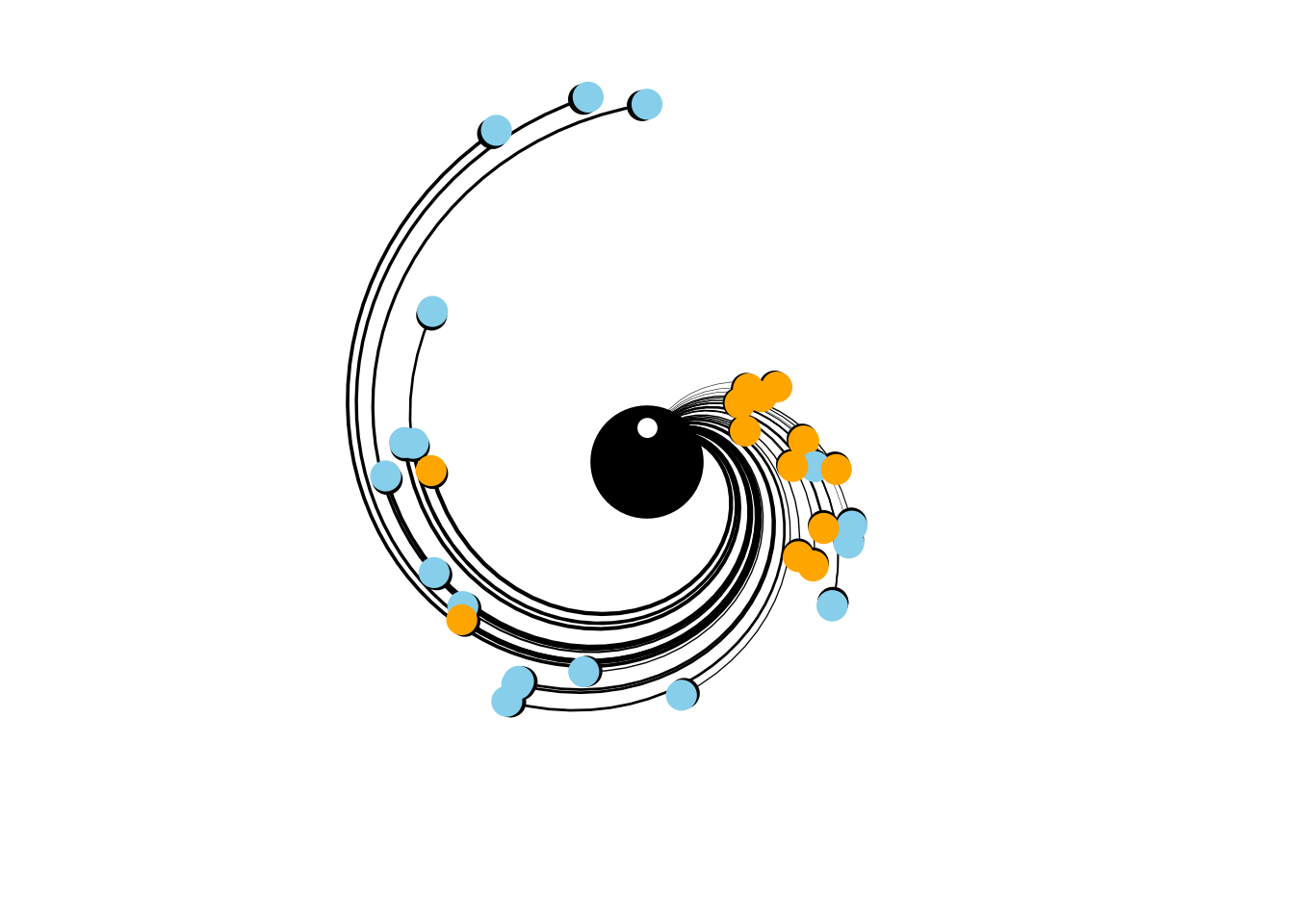
Code to create gif
gg_playback(
  name = "getting-started.gif",
  first_image_duration = 5,
  last_image_duration = 15,
  frame_duration = .7,
  image_resize = 600
)